(This page was last modified on 2/10/2019)

I tracked Jupiter during its retrograde motion in the Spring and Summer of 2016, and again in 2018.  With the results in my book this gave me six sets of values and I felt that I should be able to extract all the orbital parameters from them.  The first step was to run all the data sets through the newest version of my fitting program.  Over the years I have gradually refined the program.  I described the most recent version on the Mars page.  It allows for the possibility that the distance of the planet from the Sun can vary during the retrograde loop.  The program gives values for the distance, d, of the planet from the Sun at opposition and its angular speed, expressed as an instantaneous value of its period, T.  I can list the values I have found during all six oppositions:

Year          d (a.u.)             period, T (yrs)      longitude

2009   5.07 ± 0.08       10.9 ± 0.3              322.07°

2010    4.95 ± 0.02       10.77 ± 0.08          358.38°

2011     4.957 ± 0.006   10.80 ± 0.02         35.30°

2015    5.328 ± 0.003  12.46 ± 0.01            137.63°

2016   5.425 ± 0.003   12.91 ± 0.01             168.29°

2018  5.408 ± 0.002   12.836 ± 0.008       228.36°

Notice that the 2009 values have larger uncertainties than the later runs.  I collected that data before I had arrived at the star-field analysis method that I have used since 2010.

I came up with three ways to analyze this data.   One is similar to the approach I used to analyze the data for Venus, and  another is similar to a method I use in my book and on the Saturn/Uranus page.  But the third method was completely new, at least for me, and is, I think, illuminating, so I’ll describe it first.

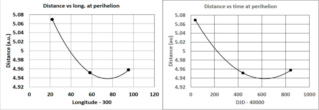
By chance the first three distances are well below my measured value of 5.20 ± 0.02 for the semi-major axis, showing that Jupiter was somewhere close to perihelion.  By design the next three were spaced around aphelion.  I can treat the two sets of points separately.  For the first three I can plot graphs of the distance versus the longitude and the distance versus time and have Excel fit parabolic curves to them.  That gives this picture:

This may sound a little simplistic, but the second-order parabola is all the data will support.  A consistency check is that the minimum value of the distance needs to be the same in both graphs, and the two values differ only slightly in the fourth decimal place.  An average of the two is 4.9385 au, and this is my estimate of the perihelion distance.  I can also read off the values of the heliocentric longitude and the time of perihelion passage  as 375°, or equivalently 15°, and a Julian date corresponding to 3/21/2011.

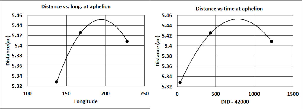
Now I can do the same thing for the three points around aphelion and this gives the figure:

The two values of the distance at the maximum again differ only in the fourth decimal place and an average is 5.4920 au, so this is my estimate of the aphelion distance.   The distance peaks at a longitude of 194.6° for the aphelion angle, corresponding to a perihelion angle of 14.6°.  The date of the maximum is 2/19/2017.  The actual time difference between the minimum in the first plot and the maximum in the second is 2,161.59 days and this is half a sidereal period.  The full period then works out to 11.84 years.  The average of the perihelion and aphelion distances is the semi-major axis, a, and from the difference of either of them from the semi-major axis I can find the eccentricity, e.

It is difficult to get a precise estimate of the uncertainties in my numbers.  As I said earlier, the 2009 values are much less precise than the others, so I can assume that is a big part of the uncertainty.  I tried changing the 2009 value of the distance by one standard deviation and running all the calculations again.  The biggest change was in the perihelion angle, which shifted by over 4°, and, to a lesser extent, the perihelion distance, which was increased to 4.9491 au.  With this as a guide I estimate my results as

a = 5.195 ± 0.005 au,     e = 0.049 ± 0.001,    perihelion longitude = 14.6 ± 1.0°

For the perihelion longitude I have relied on the aphelion longitude from the second set of points.

Before I hit on this approach I had attempted to use a variation of the method I used on the Venus page to find its orbit parameters, that is, a non-linear least squares fit of the orbit parameters to the six sets of distances and heliocentric longitudes.  The catch was that for Venus I already had a very precise value for the semi-major axis so that I was fitting only two parameters, the eccentricity and the longitude at perihelion.  For Jupiter I attempted to fit the semi-major axis as well.  Fitting three parameters to six data points is asking a lot of a non-linear fit, and even for Venus I had to pin down the minimum by searching through a fine grid of values before starting the fit.  For Jupiter I set up a fine grid of parameter values in Excel and located the  minimum of the quality of fit parameter, χ, as coming close to the values a = 5.199 au,  e = 0.0492, and longitude at perihelion = 14.9°.  In fact, when I started the non-linear fit at these values it produced a negligible change in the numbers and drifted around for a rather ridiculous 300 iterations of the fitting process.  So the values I got from the grid are the best I can get out of this method.  They are, happily, close to the values from the previous method.  The reason I attempted the fitting process was that the formulas also give uncertainties on the parameter values, and I wanted those.  But I felt that the fit was so ill-conditioned that the uncertainties were probably meaningless.

So neither of these two methods gave me a firm handle on the uncertainties, and I also felt that the less-accurate early data sets were contributing too much to the final results.  The third method is one that I used in my book and also for Saturn and Uranus on their page.  It is based on calculating the ratio d²/T for each year’s values.  I pointed out in the book that Kepler’s second law is equivalent to this ratio being a constant of the motion and I did verify that it was constant within the uncertainties.  The values that I now calculate are

Year                    d²/T

2009                 2.35 ± 0.10

2010                  2.276 ± 0.026

2011                   2.2753 ± 0.0065

2015                  2.2779 ± 0.0033

2016                  2.2794 ± 0.0084

2018                  2.2787 ± 0.0018

In previous use of this ratio I have, rather casually, chosen the value with the smallest uncertainty.  But there is a well defined statistical procedure for calculating an average weighting each term according to its precision, called a best linear unbiassed estimate.  It is, after all, the best value.  For the numbers above it comes out as 2.2783 ± 0.0018. For an elliptical orbit satisfying Kepler’s laws it is equal to a²√(1 – e²)/P.  I do need to take the value of e from my first analysis method as 0.049, but the factor √(1-e²) is so close to 1 that its uncertainty doesn’t matter.  Then the ratio a²/P is 2.2810 ± 0.0018.  If If I combine this with Kepler’s third law I can show that this ratio equals either the square root of a or the cube root of P, so that

a = 5.203 ± 0.008 au, and P = 11.87 ± 0.03 years.

These values, with their uncertainties, are the ones I have the most confidence in, combined with the values e = 0.049 ± 0.001 and  longitude at perihelion = 14.6 ± 1° from the first method.  I described my calculation of the tilt of the orbit from the ecliptic and the longitude of the ascending node in chapter 15 of my book, and the mass of Jupiter, based on the orbits of its moons, in chapter 20.

Here is a small thought to finish this page with.  I always try to make my measurements and calculations without being too much influenced by the values given in the handbooks.  But I am not so sure of myself that I don’t compare my numbers with the handbook afterwards.  The Observer’s Handbook lists the orbital parameters for each planet at the beginning of each year and six months into the year, and the numbers do change slightly.  They represent the best fit to an ellipse at that time for an orbit that is not exactly elliptical.  I notice that in the case of Jupiter my uncertainties are getting down towards the variations in the parameter values .  This implies that, to improve my results much beyond what I now have, I shall have to give up the strong reliance on Kepler’s laws that I have been accustomed to!